2 Unidimensional Exploration

In this first section, we focus on the exploration of one dimension of the data.cube. Multidimensional exploration is demonstrated later.

2.1 Selecting one dimension with select.dim

One first needs to select the dimension of interest using function select.dim. In this example, we focus on the dataset’s temporal dimension, a.k.a. dimension week.

geomedia %>%
    select.dim (week) %>%
    as.data.frame ()

## # A tibble: 79 x 2
##    week       articles
##    <date>        <dbl>
##  1 2015-06-01    5706.
##  2 2015-03-09    6316.
##  3 2014-05-19    5857.
##  4 2014-10-13    6006.
##  5 2014-06-09    5172.
##  6 2015-06-22    6738.
##  7 2015-01-05    5607.
##  8 2014-05-26    5260.
##  9 2015-05-04    6368.
## 10 2014-06-16    3384.
## # … with 69 more rows

The resulting data.cube consists in a unidimensional data structure where variable articles has been aggregated (summed) along dimensions media and country. The resulting data.frame hence gives the total number of published articles corresponding to each element of dimension week.

2.2 Arranging elements with arrange.elm

Note that above, observations have no particular order. Function arrange.elm reorders elements of a given dimension according to one (or several) of their variables. For example, the lexicographic order of their name (standard variable created for each dimension when instantiating the data.cube) which happens to also be the chronological order.

geomedia %>%
    select.dim (week) %>%
    arrange.elm (week, name) %>%
    as.data.frame ()

## # A tibble: 79 x 2
##    week       articles
##    <date>        <dbl>
##  1 2013-12-30    1671.
##  2 2014-01-06    2983.
##  3 2014-01-13    3172.
##  4 2014-01-20    3519.
##  5 2014-01-27    3073.
##  6 2014-02-03    2972.
##  7 2014-02-10    3012.
##  8 2014-02-17    2881.
##  9 2014-02-24    3313.
## 10 2014-03-03    3573.
## # … with 69 more rows

2.3 Plotting variables with plot.var

Function plot.var then plots a variable. Note that it returns a ggplot object that can hence be modified using classical tools of the visualisation library. For example, one can use function theme to vertically display x-axis labels.

geomedia %>%
    select.dim (week) %>%
    arrange.elm (week, name) %>%
    plot.var (articles) +
    theme (axis.text.x = element_text (angle = 90, size = 6))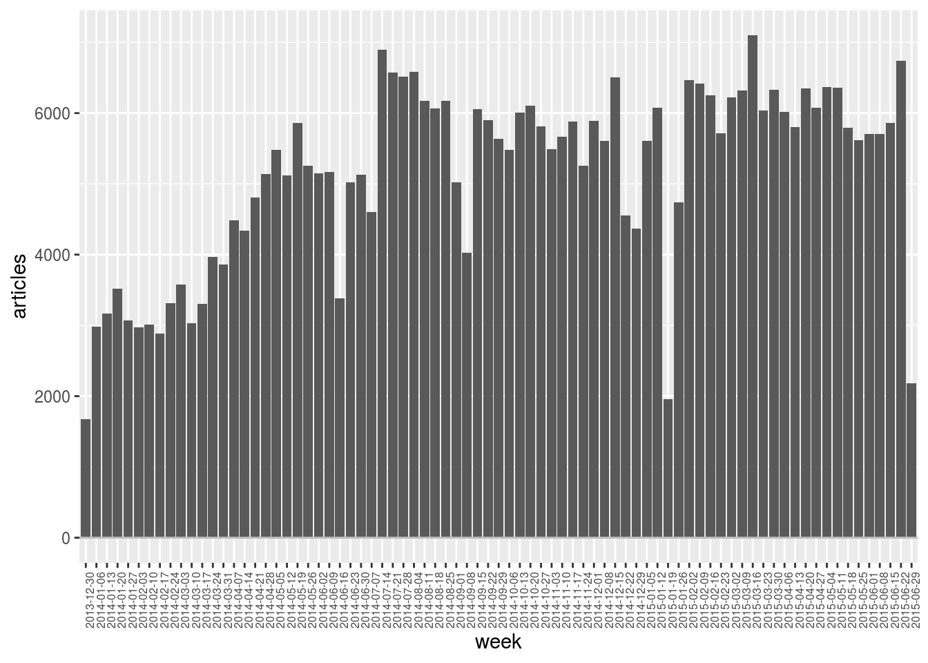

Several plot types are available: bar (above), line (below), and point.

geomedia %>%
    select.dim (week) %>%
    arrange.elm (week, name) %>%
    plot.var (articles, type = "line") +
    theme (axis.text.x = element_text (angle = 90, size = 6))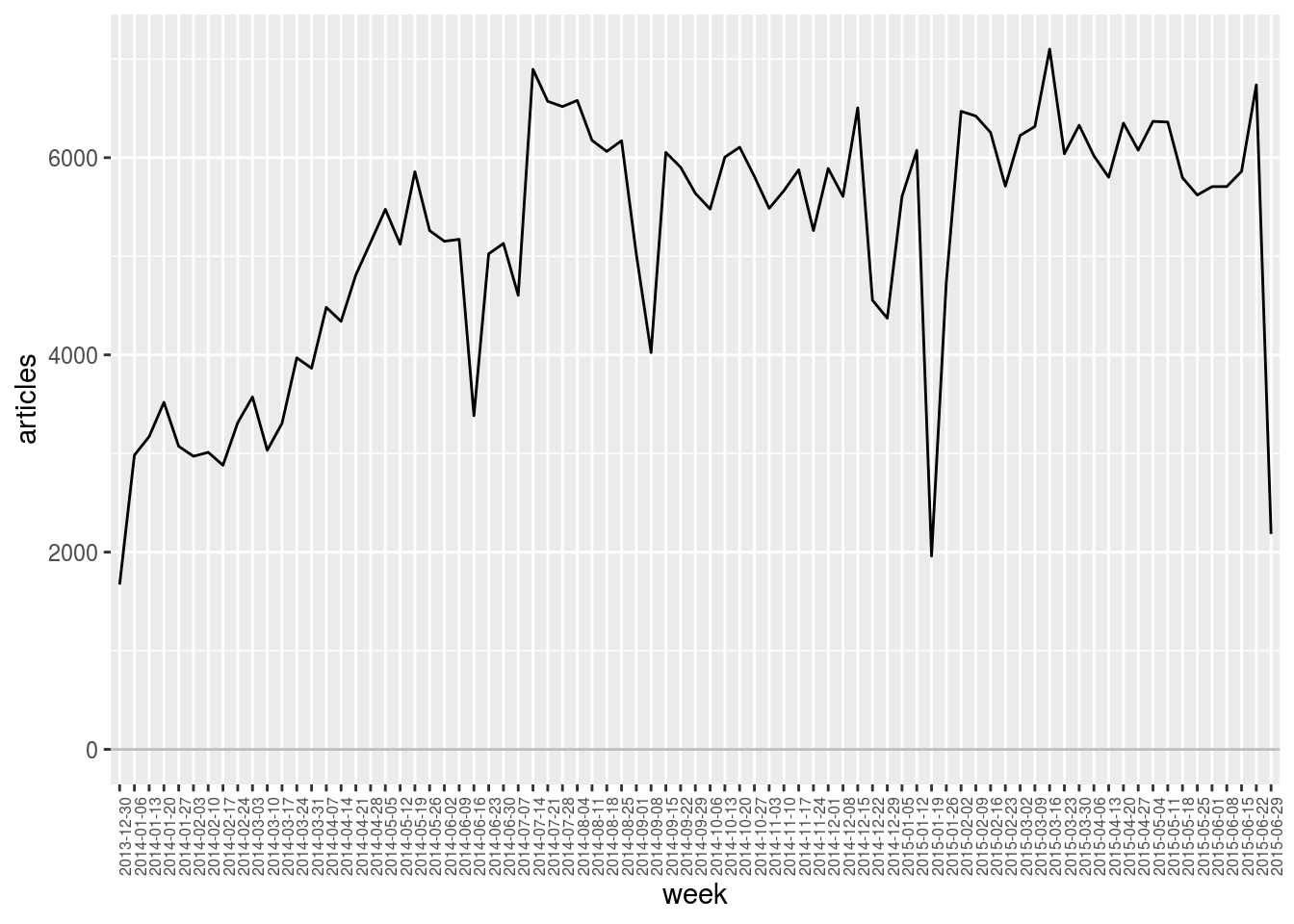

2.4 Filtering elements with filter.elm and top_n.elm

Note that some observations in the plot above are surprisingly low. (They actually correspond to technical incidents during data collection.)

Function top_n.elm only keeps the elements of a dimension that have the highest (or the lowest) value according to a variable. We here plot the 10 weeks in the data that have the lowest number of published article (note the - in argument n).

geomedia %>%
    select.dim (week) %>%
    top_n.elm (week, articles, n = -10) %>%
    arrange.elm (week, articles) %>%
    plot.var (articles) +
    theme (axis.text.x = element_text (size = 6))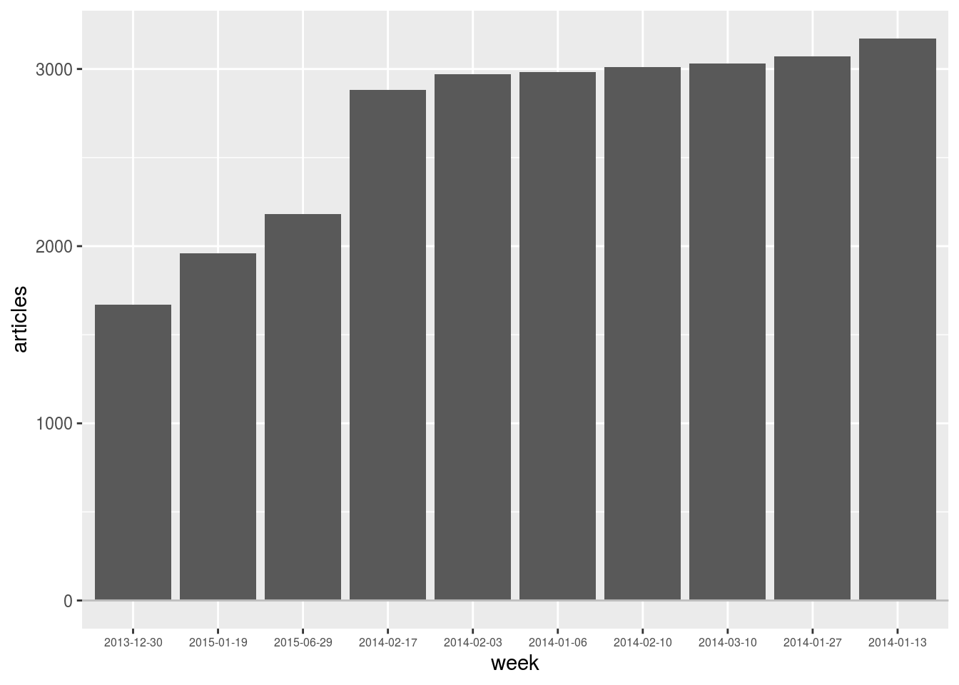

Function filter.elm only keeps the elements of a dimension that fit with some criteria expressed on variables. We can for example use it to remove such anomalous observations.

geomedia %>%
    select.dim (week) %>%
    filter.elm (week, articles >= 2500) %>%
    arrange.elm (week, name) %>%
    plot.var (articles, type = "line") +
    theme (axis.text.x = element_text (angle = 90, size = 6))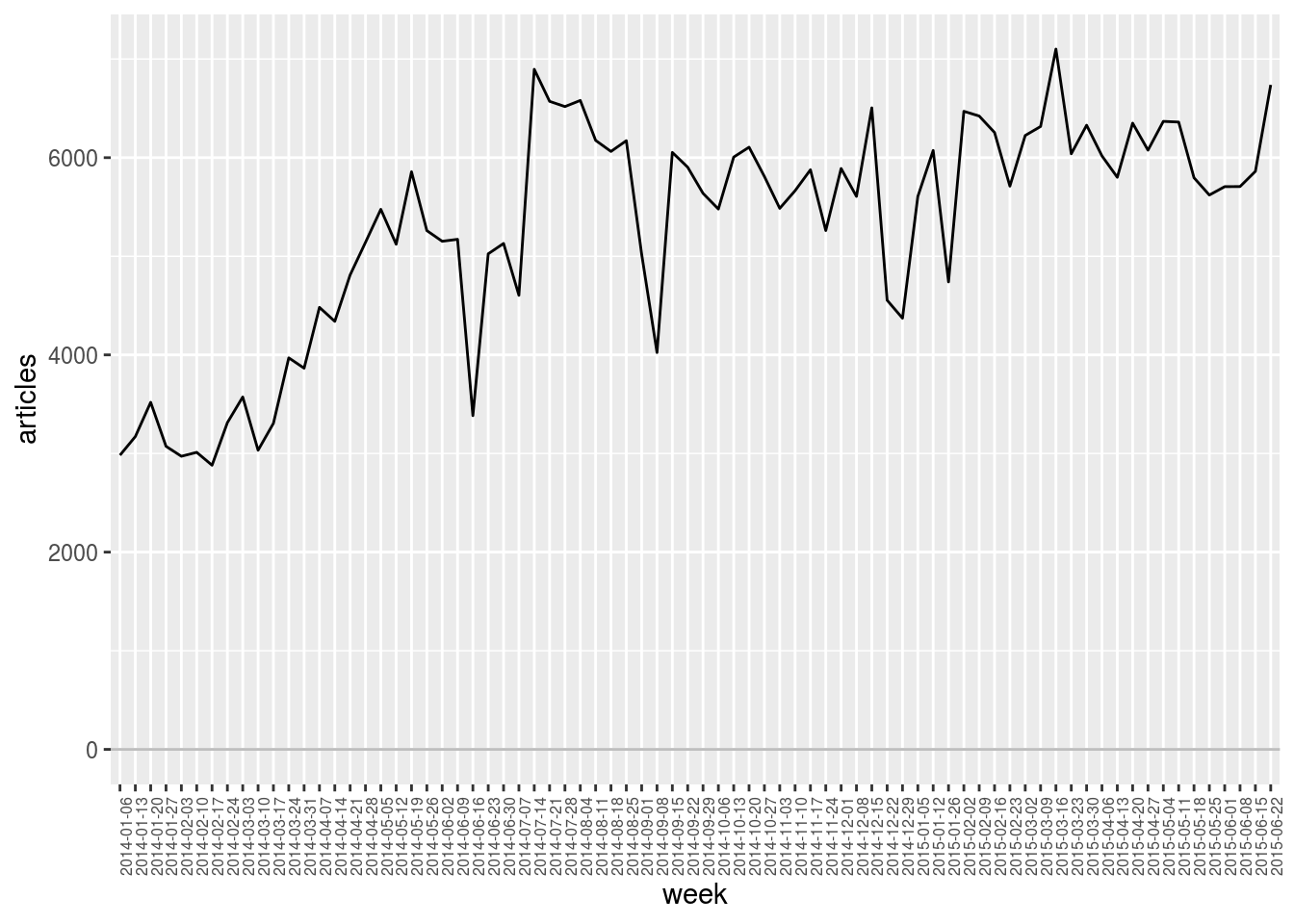

2.5 Other examples of use

Here are other examples of use of these simple operations, illustrated on the spatial dimension country.

One can plot the number of articles associated with the top 20 countries (arranged in a decreasing order).

geomedia %>%
    select.dim (country) %>%
    top_n.elm (country, articles, 20) %>%
    arrange.elm (country, desc (articles)) %>%
    plot.var (articles)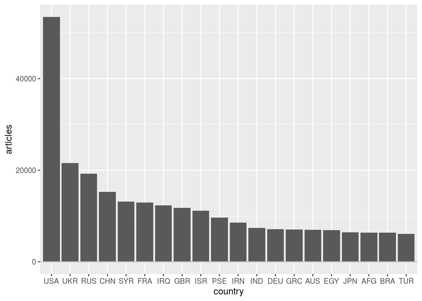

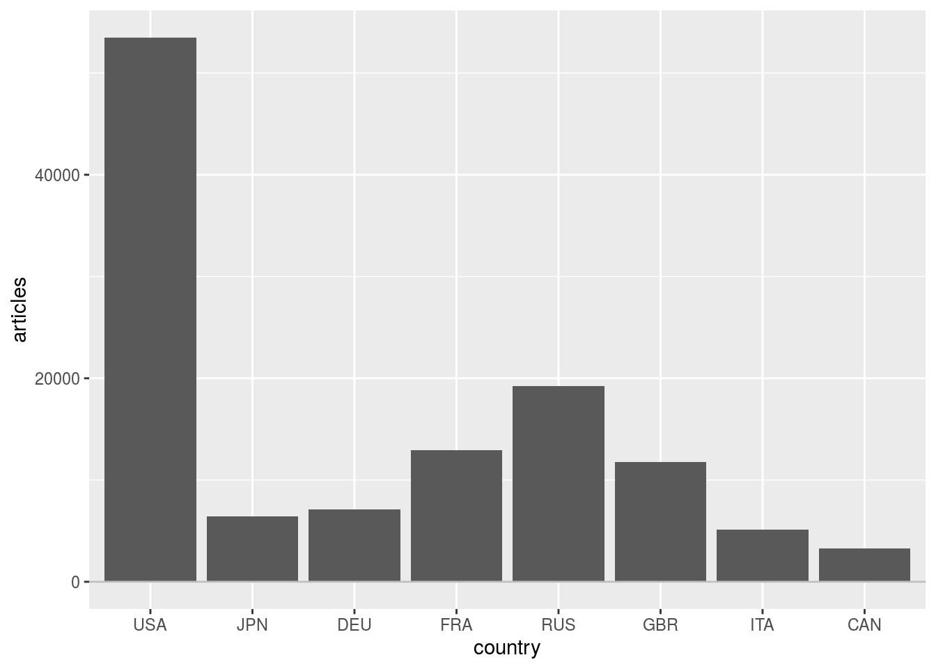
One can filter and arrange countries according to a given subset.

G8 <- c ("USA", "JPN", "DEU", "FRA", "RUS", "GBR", "ITA", "CAN")
geomedia %>%
    select.dim (country) %>%
    filter.elm (country, name %in% G8) %>%
    arrange.elm (country, match (name, G8)) %>%
    plot.var (articles)